Prediction of Labour Force Size in Malaysia using Linear Regression
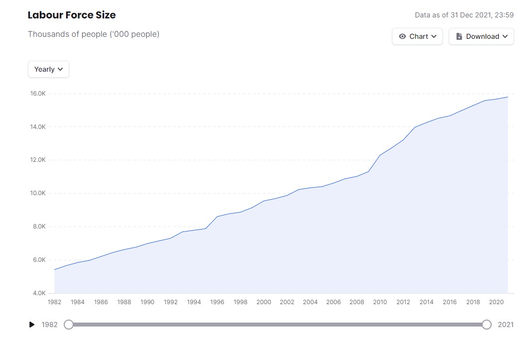
A simple linear regression model using Scikit-Learn to predict the annual labour size in Malaysia. I found this model is suitable for this dataset as the actual data is already considerably linear.
This dataset was imported from OpenDOSM, an open-sourced website by Department of Statistics Malaysia. It is based on The Labour Force Survey (LFS) from the year 1982 to 2021. However, there is no data for 1991 and 1994 because the LFS was not conducted in those years. The sum of each category may not always equal to the totals shown in related tables because of independent rounding to one decimal place.
import numpy as np
import pandas as pd
import math as math
from sklearn.linear_model import LinearRegression
from sklearn.model_selection import train_test_split
lbforce_df = pd.read_csv("labour-principalstats-annual.csv")
lbforce_df.head()
| date | lf_size | employed | unemployed | outside | u_rate | p_rate | ep_ratio | |
|---|---|---|---|---|---|---|---|---|
| 0 | 1982-01-01 | 5431.4 | 5249.0 | 182.4 | 2944.6 | 3.4 | 64.8 | 62.67 |
| 1 | 1983-01-01 | 5671.8 | 5457.0 | 214.9 | 2969.4 | 3.8 | 65.6 | 63.15 |
| 2 | 1984-01-01 | 5862.5 | 5566.7 | 295.8 | 3119.6 | 5.0 | 65.3 | 61.98 |
| 3 | 1985-01-01 | 5990.1 | 5653.4 | 336.8 | 3124.9 | 5.6 | 65.7 | 62.02 |
| 4 | 1986-01-01 | 6222.1 | 5760.1 | 461.9 | 3188.3 | 7.4 | 66.1 | 61.21 |
lbforce_df.describe()
| lf_size | employed | unemployed | outside | u_rate | p_rate | ep_ratio | |
|---|---|---|---|---|---|---|---|
| count | 38.000000 | 38.000000 | 38.000000 | 38.000000 | 38.000000 | 38.000000 | 38.000000 |
| mean | 10300.115421 | 9917.558211 | 382.573026 | 5336.476763 | 3.877928 | 65.701364 | 63.146842 |
| std | 3299.374363 | 3219.000270 | 119.341681 | 1543.031558 | 1.244466 | 1.706195 | 1.695139 |
| min | 5431.400000 | 5249.000000 | 182.400000 | 2944.600000 | 2.400000 | 62.600000 | 60.550000 |
| 25% | 7414.275000 | 7131.700000 | 314.075000 | 3806.425000 | 3.200000 | 64.425000 | 61.990000 |
| 50% | 10062.870500 | 9706.180000 | 368.300000 | 5466.171500 | 3.400000 | 65.600000 | 62.690000 |
| 75% | 13101.450000 | 12703.250000 | 446.500000 | 6857.675000 | 4.025000 | 66.725000 | 64.472500 |
| max | 15797.200000 | 15073.400000 | 733.000000 | 7225.500000 | 7.400000 | 68.700000 | 66.400000 |
lbforce_df.info()
<class 'pandas.core.frame.DataFrame'>
RangeIndex: 38 entries, 0 to 37
Data columns (total 8 columns):
 #   Column      Non-Null Count  Dtype
---  ------      --------------  -----
 0   date        38 non-null     object
 1   lf_size     38 non-null     float64
 2   employed    38 non-null     float64
 3   unemployed  38 non-null     float64
 4   outside     38 non-null     float64
 5   u_rate      38 non-null     float64
 6   p_rate      38 non-null     float64
 7   ep_ratio    38 non-null     float64
dtypes: float64(7), object(1)
memory usage: 2.5+ KB
# Create a separate column for year, set Dtype as float and reshape the series as a numpy array
lbforce_df['year'] = lbforce_df['date'].str[:4].astype(float)
year = lbforce_df[['year']]
year = year.values
lbforce_df.info()
<class 'pandas.core.frame.DataFrame'>
RangeIndex: 38 entries, 0 to 37
Data columns (total 9 columns):
 #   Column      Non-Null Count  Dtype
---  ------      --------------  -----
 0   date        38 non-null     object
 1   lf_size     38 non-null     float64
 2   employed    38 non-null     float64
 3   unemployed  38 non-null     float64
 4   outside     38 non-null     float64
 5   u_rate      38 non-null     float64
 6   p_rate      38 non-null     float64
 7   ep_ratio    38 non-null     float64
 8   year        38 non-null     float64
dtypes: float64(8), object(1)
memory usage: 2.8+ KB
print(year)
[[1982.]
 [1983.]
 [1984.]
 [1985.]
 [1986.]
 [1987.]
 [1988.]
 [1989.]
 [1990.]
 [1992.]
 [1993.]
 [1995.]
 [1996.]
 [1997.]
 [1998.]
 [1999.]
 [2000.]
 [2001.]
 [2002.]
 [2003.]
 [2004.]
 [2005.]
 [2006.]
 [2007.]
 [2008.]
 [2009.]
 [2010.]
 [2011.]
 [2012.]
 [2013.]
 [2014.]
 [2015.]
 [2016.]
 [2017.]
 [2018.]
 [2019.]
 [2020.]
 [2021.]]
# Assign independent (x) and dependent (y) variables
x = year
y = lbforce_df.iloc[:, 1]
# Divide the dataset into training and testing dataset
x_train, x_test, y_train, y_test = train_test_split(x, y, test_size = 0.3, random_state = 0)
# Apply the linear regression algorithm
simplelinearRegression = LinearRegression()
simplelinearRegression.fit(x_train, y_train)
LinearRegression()In a Jupyter environment, please rerun this cell to show the HTML representation or trust the notebook.
On GitHub, the HTML representation is unable to render, please try loading this page with nbviewer.org.
LinearRegression()
y_predict = simplelinearRegression.predict(x_test)
predict = pd.DataFrame(y_predict)
predict.apply(np.round)
| 0 | |
|---|---|
| 0 | 11455.0 |
| 1 | 13380.0 |
| 2 | 9805.0 |
| 3 | 9529.0 |
| 4 | 8429.0 |
| 5 | 10905.0 |
| 6 | 12555.0 |
| 7 | 7879.0 |
| 8 | 12280.0 |
| 9 | 5404.0 |
| 10 | 13930.0 |
| 11 | 14480.0 |
Using the predict function, we pass the tested value of the 'x' variable (year) and we get the predicted values (labour force size). Now we try to predict the values within the range of our dataset and compare it with real data.
print("Prediction of Annual Labour Force Size in Malaysia ('000 people)")
i = 2011
while i <= 2021:
    print("Year %d ==>" %(i), int(simplelinearRegression.predict([[i]])))
    i= i+1
Prediction of Annual Labour Force Size in Malaysia ('000 people)
Year 2011 ==> 12829
Year 2012 ==> 13104
Year 2013 ==> 13379
Year 2014 ==> 13654
Year 2015 ==> 13929
Year 2016 ==> 14204
Year 2017 ==> 14479
Year 2018 ==> 14754
Year 2019 ==> 15030
Year 2020 ==> 15305
Year 2021 ==> 15580
print("Actual Labour Force Size in Malaysia ('000 people)")
print(lbforce_df.iloc[30:38, 0:2])
Actual Labour Force Size in Malaysia ('000 people)
          date  lf_size
30  2014-01-01  14263.6
31  2015-01-01  14518.0
32  2016-01-01  14667.8
33  2017-01-01  14980.1
34  2018-01-01  15280.3
35  2019-01-01  15581.6
36  2020-01-01  15667.7
37  2021-01-01  15797.2
The predicted values are considerably close to the real annual labour size. Now we try to predict beyond our dataset range.
print("Prediction of Annual Labour Force Size in Malaysia ('000 people)")
i = 2022
while i <= 2035:
    print("Year %d ==>" %(i), int(simplelinearRegression.predict([[i]])))
    i= i+1
Prediction of Annual Labour Force Size in Malaysia ('000 people)
Year 2022 ==> 15855
Year 2023 ==> 16130
Year 2024 ==> 16405
Year 2025 ==> 16680
Year 2026 ==> 16955
Year 2027 ==> 17230
Year 2028 ==> 17505
Year 2029 ==> 17780
Year 2030 ==> 18055
Year 2031 ==> 18330
Year 2032 ==> 18605
Year 2033 ==> 18880
Year 2034 ==> 19155
Year 2035 ==> 19430